IIR Filter

IIR filter stands for Infinite Impulse Response. Such filters have feedback so that signals are processed in a recursive way. We will see that impulse responses from exponentials can easily be implemented as a recursive filter.

Introduction

As an instructional example we take a very simple analogue filter and sample it. This can then be generalised to more complex situations.

We define a first order filter which can be implemented, for example, as a simple RC network:

  $$h(t)=e^{-bt}$$ (151)

where its Laplace transform is a simple fraction:

  $$H(s)=\frac{1}{s+b}$$ (152)

Now we sample Eq. 151:

  $$h(t)=\sum_{n=0}^\infty e^{-bnT} \cdot \delta(t-nT)$$ (153)

and perform a Laplace transform on it:

  $$H(s) = \sum_{n=0}^\infty e^{-bnT} \underbrace{e^{-nsT}}_{{z^{-1}}^n}$$ (154)

which turns into a z-transform:

$$H(z) = \sum_{n=0}^\infty e^{-bnT} z^{-n}$$ (155)

$$= \sum_{n=0}^\infty {\left(e^{-bT} z^{-1}\right)}^n$$ (156)

$$= {1\over 1-e^{-bT} z^{-1}}$$ (157)

Consequently the analogue transfer function $H(s)$ transfers into $H(z)$ with the following recipe:

  $$H(s)=\frac{1}{s+b} \qquad\Leftrightarrow\qquad H(z)=\frac{1}{1-e^{-bT} z^{-1}}$$ (158)

Thus, if you have the poles of an analogue system and you want to have the poles in the z-plane you can transfer them with:

  $$z_\infty=e^{s_\infty T}$$ (159)

This also gives us a stability criterion. In the Laplace domain the poles have to be in the left half plane (real value negative). This means that in the sampled domain the poles have to lie within the unit circle.

The same rule can be applied to zeros

  $$z_0=e^{s_0 T}$$ (160)

together with Eq. 159 this is called “The matched z-transform method”. For example $H(s)=s$ turns into $H(z)=1-z^{-1}e^{0T}=1-z^{-1}$ which is basically a DC filter.

Determining the data-flow diagram of an IIR filter

Figure 21: IIR filter

To get a practical implementation of Eq. 157 we have to see it with its input- and output-signals:

$$Y(z) = X(z)H(z)$$ (161)

$$= X(z) {1\over 1-e^{-bT} z^{-1}}$$ (162)

$$= Y(z)z^{-1}e^{-bT}+X(z)$$ (163)

We have to recall that $z^{-1}$ is the delay by $T$. With that information we directly have a difference equation in the temporal domain:

  $$y(nT)=y([n-1]T) e^{-bT} + x(nT)$$ (164)

This means that the output signal $y(nT)$ is calculated by adding the weighted and delayed output signal $y([n-1]T)$ to the input signal $x(nT)$. How this actually works is shown in Fig. 21. The attention is drawn to the sign inversion of the weighting factor $e^{-bT}$ in contrast to the transfer function Eq. 158 where it is $-e^{-bT}$. In general the recursive coefficients change sign when they are taken from the transfer function.

General form of IIR filters

A filter with forward and feedback components can be represented as:

  $$H(z) = \frac{\sum_{k = 0}^{r} B_{k} z^{-k}}{1 + \sum_{l = 1}^{m} A_{i} z^{-l}}$$ (165)

where $B_k$ are the FIR coefficients and $A_l$ the recursive coefficients. Note the signs of the recursive coefficients are inverted in the actual implementation of the filter. This can be seen when the function $H(z)$ is actually multiplied with an input signal to obtain the output signal (see Eq. 164 and Fig. 21). The “1” in the denominator represents actually the output of the filter. If this factor is not one then the output will be scaled by that factor. However, usually this is kept one.

In Python filtering is performed with the command:

import scipy.signal as signal
Y = signal.lfilter(B,A,X)

where B are the FIR coefficients, A the IIR coefficients and X is the input. For a pure FIR filter we just have:

Y = signal.lfilter(B,1,X)

The “1” represents the output.

IIR filter topologies

Figure 22: A) Direct Form I filter which one accumulator and B) Direct Form II filter with two accumlators.

In real applications one would create a chain of 2nd order IIR filters. This has numerous advantages:

1. The optimisation can be done within these simple structures, for example omitting array operations completely and coding the 2nd order filters in assembly while keeping the higher level operations in C or C++.
2. Control of stability issues: high order recursive systems might become unstable and it is very hard to predict when this might happen. On the other hand a chain of 2nd order filters can be made stable with ease. One can focus on stability in 2nd order systems which is well understood and manageable.
3. Complex conjugate pole pairs are generated naturally in analogue filter design and directly translate to 2nd order IIR structures. Analogue design is usually described as 2nd order structures (=LCR) so that any transform from analogue to digital just needs to be of 2nd order!

Fig. 22 shows the most popular filter topologies: Direct Form I and II. Because of the linear operation of the filter one is allowed to do the FIR and IIR operations in different orders. In Direct From I we have one accumulator and two delay lines whereas in the Direct Form II we have two accumulators and one delay line. Only the Direct Form I is suitable for integer operations.

A Python class of a direct form II filter can be implemented with a few lines:

class IIR_filter:
    def __init__(self,_num,_den):
        self.numerator = _num
        self.denominator = _den
        self.buffer1 = 0
        self.buffer2 = 0

    def filter(self,v):
        input=0.0
        output=0.0
        input=v
        output=(self.numerator[1]*self.buffer1)
        input=input-(self.denominator[1]*self.buffer1)
        output=output+(self.numerator[2]*self.buffer2)
        input=input-(self.denominator[2]*self.buffer2)
        output=output+input*self.numerator[0]
        self.buffer2=self.buffer1
        self.buffer1=input
        return output

Here, the two delay steps are represented by two variables buffer1 and buffer2.

In order to achive higher order filters one can then just chain these 2nd order filters. In Python this can be achieved by storing these in an array of instances of this class.

Fixed point IIR filters

Figure 23: Direct Form I filter with fixed point arithmetic.

Fig. 23 shows the implementation of a fixed point IIR filter. It's a Direct Form I filter with one accumulator so that temporary overflows can be compensated. The original floating point IIR coefficients are scaled up by factor $2^w$ so that they max out the range of the integer coefficients. After the addition operation they are shifted back by $w$ bits to their original values.

For example if the largest IIR coefficient is 1.9 and we use 16 bit signed numbers (max number is 32767) then one could multiply all coefficients with $2^{14}$.

Then one needs to assess the maximum value in the accumulator which is much more difficult than for FIR filters. For example, resonators can generate high output values with even small input values so that it's advisable to have a large overhead in the accumulator. For example if the input signal is $16$ bit and the scaling factor is $14$ bits then the signal will certainly occupy $16+14=30$ bits. With an accumulator of 32 bits that gives only a headroom of 2 bits so the output can only be 4 times larger than the input. A 64 bit accumulator is a safe bet.

Filter design based on analogue filters

Figure 24: Pole placements of the Butterworth filter. Its analogue cutoff frequency is $\Omega = 2\pi F$ where $F$ is the analogue cutoff frequency in Hertz. This filter can be implemented as a chain of 2nd order IIR filters (biquads) by using the complex conjugate pairs for the different 2nd order IIR filters.

Most IIR filters are designed from analogue filters by transforming from the continuous domain ($h(t),H(s)$) to the sampled domain ($h(n),H(z)$).

A list of popular analogue transfer functions being used for IIR filter design:

• Butterworth: All poles lie on the left half plane equally distributed on a half circle with radius $\Omega = 2\pi F$ which is shown in Fig. 24. The Butterworth filter is by far the most popular filter. Here are its properties:
  • monotonic frequency response
  • only poles, no zeros
  • the Poles have analytical solution and very easy to calculate
  • no constant group delay but usually acceptable deviation from a strict constant group delay for many applications.

• Chebyshev Filters:
    $$\vert H(\Omega)\vert^{2} = \frac{1}{1 - \varepsilon^{2} T_{N} (\Omega/\Omega_{p})}$$ (166)
  where T = Chebyslev polynomials. These filters have either ripples in the stop or passband depending on the choice of polynomials. As with Butterworth the polynomials have analytical solutions for the poles and zeros of the filter so that their design again is straightforward.

• Bessel Filter:
  • Constant Group Delay
  • Shallow transition from stop- to passband
  • No analytical solution for the poles/zeros.

How to transform the analogue lowpass filters into highpass, bandstop or bandpass filters?

All the analogue transfer functions above are lowpass filters. However this is not a limitation because there are handy transforms which take an analogue lowpass transfer function or poles/zeros and then transforms them into highpass, bandpass and stopband filters. These rules can be found in any good analogue filter design book and industry handouts, for example from Analog Devices.

Bilinear Transform: transforming the analoge transfer function into a digital one:

As a next step these analogue transfer functions $H(s)$ need to be transformed to digital transfer functions $H(z)$. This could be done by the matched z-transform (Eq. 160). However, the problem with these methods is that they map frequencies 1:1 between the digital and analogue domain. Remember: in the sampled domain there is no infinite frequency but $F_s/2$ which is the Nyquist frequency. This means that we never get more damping than at Nyquist $F_s/2$. This is especially a problem for lowpass filters where damping increases the higher the frequency.

The solution is to map all analogue frequencies from $0 \ldots \infty$ to the sampled frequencies $0\ldots 0.5$ in a non-linear way:

  $$- \infty < \Omega < \infty \Rightarrow -\pi \leq \omega \leq \pi$$ (167)

This is called Bilinear Transformation:

  $$s = \frac{2}{T} \quad \frac{z - 1}{z + 1}$$ (168)

This rule replaces all $s$ with $z$ in our analogue transfer function so that it's now digital. However, the cutoff frequency $\Omega_c$ is still an analogue one but if we want to design a digital filter we want to specify a digital cutoff frequency. Plus remember that the frequency mapping is non-linear so that there is non-linear mapping also of the cutoff.

In the analogue domain the frequency is given as $s = j\Omega$ and in the sampled domain as $z = e^{j \omega}$. With the definition of the bilinear transform we can establish how to map from our desired digital cutoff to the analogue one:

  $$j \Omega = \frac{2}{T} \left[\frac{e^{j \omega} - 1}{e^{j \omega} +1}\right] = \frac{2}{T} j \tan \frac{\omega}{2}$$ (169)

This derivation is useful for two purposes. It shows the non-linear mapping between the digital and analogue world and it provides a recipe how to calculate our analogue cutoff frequency.

That the bilinear transform is a nonlinear mapping between the analogue world and the digital world can be directly seen by just omitting the $j$:

  $$\Omega = \frac{2}{T} tan \frac{\omega}{2}$$ (170)

This also means that the cut-off frequency of our analogue filter is changed by the bilinear transformation. Consequently, we need to apply the same transformation to the cutoff frequency itself:

  $$\Omega_{c} = \frac{2}{T} tan \frac {\omega_{c}}{2}$$ (171)

where $T$ is the sampling interval. This is often called “pre-warp” but is simply the application of the same rule to the cut-off frequency as what the bilinear transform does to the transfer function $H(s)$. It has also another important result: we can now finally specify our cut-off in the sampled domain in normalised frequencies $\omega_{c} = 2\pi f_{c}$ by using Eq. 171. After all we just use the analogue filter as a vehicle to design a digital filter.

We can now list our design steps.

IIR filter design steps:

1. Choose the cut-off frequency of your digital filter $\omega_{c}$.
2. Calculate the analogue cutoff frequency $\omega_{c} \rightarrow \Omega_{c}$ with Eq. 171
3. Choose your favourite analogue lowpass filter $H(s)$, for example Butterworth.
4. Replace all $s$ in the analogue transfer function $H(s)$ by $s = \frac{2}{T} \frac{z - 1}{z + 1}$ to obtain the digital filter $H(z)$
5. Change the transfer function $H(z)$ so that it only contains negative powers of $z$ ( $z^{-1}, z^{-2}, \ldots$) which can be interpreted as delay lines.
6. Build your IIR filter!

For filter-orders higher than two one needs to develop a different strategy because the bilinear transform is a real pain to calculate for anything above the order of two. Nobody wants to transform high order analogue transfer functions $H(s)$ to the $H(z)$ domain. However, there is an important property of all analogue transfer functions: they generate complex conjugate pole pairs (plus one real pole if of of odd order) which suggest a chain of 2nd order IIR filters straight away (see Fig. 24). Remember that a complex conjugate pole pair creates a 2nd order IIR filter with with two delay steps. A real pole is a 1st order IIR filter with one delay but is often also implemented as a 2nd order filter where the coefficients of the 2nd delay are kept zero.

The design strategy is thus to split up the analogue transfer function $H(s)$ in a chain of 2nd order filters $H(s) = H_1(s) H_2(s) H_3(s) \ldots$ and then to apply the bilinear transform on every 2nd order term separately. Using this strategy you only need to calculate the bilinear transform once for a 2nd order system (or if the order is odd then also for a 1st order one) but then there is no need to do any more painful bilinear transforms. This is standard practise in IIR filter design.

Time or frequency domain?

The transforms from analogue to digital alter both the temporal response and the frequency response. However the different transforms have different impact. The bilinear transform guarantees that the digital filter uses the whole frequency range of the analogue filter from zero to infinity which is the best solution for frequency domain problems. However, if one needs to reproduce the temporal response an analogue filter as faithfully as possible then the matched z transform is best because it's based (as the name suggests) on the impulse invariance method which aims to preserve the temporal behaviour of the filter (exact for pole-only transfer functions).

Identical frequency response required:	Bilinear transform
Identical temporal behaviour required:	Matched z-transform

Of course a 100% match won't be achieved but in practise this can be assumed. In most cases the bilinear transform is the transform of choice. The matched z transform can be very useful, for example in robotics where timing is important.

Adaptive IIR filter: The Kalman filter

Often signals are contaminated by high frequency noise where the spectrum of the noise is changing or not known. The cutoff of a fixed low pass filter is not known or might be changing so that we need to adapt the cut-off continuously. One example is a Kalman filter which maximises the predictability of the filtered signal. It's an adaptive lowpass filter which increases the predictability of a signal because it smoothes it.

  $$H(z) = \frac{b}{1 - a z^{-1}}$$ (172)

The parameter $a$ determines the cutoff frequency. Frequency Response :

  $$\vert H(e^{j \omega}) \vert = \vert\frac{b}{1 - a e^{-j \omega}}\vert$$ (173)

Let's re-interpret our low-pass filter in the time domain:

  $$\underbrace{y(n)}_{\mbox {\footnotesize actual estimate}} = a(n) ... ...estimate}} + b(n)\underbrace{x(n)}_{\mbox{\footnotesize current data sample}}$$ (174)

We would like to have the best estimate for $y(n)$

  $$p(n) = E[ \left( y (k) - y_{real} (k)\right)^{2}]$$ (175)

We need to minimise $p$ which gives us equations for a and b which implements a Kalman filter.

The role of poles and zeros

Transfer functions contain poles and zeros. To gain a deeper understanding of the transfer functions we need to understand how poles and zeros shape the frequency response of $H(z)$. The position of the poles also determines the stability of the filter which is important for real world applications.

We are going to explore the roles of poles and zeros first with an instructional example which leads to a 2nd order bandstop filter.

Zeros

Figure 25: A two tap FIR stopband filter for the frequency $\omega _0$.

Let's look at the transfer function:

$$H(z) = (1 - e^{j\omega_0} z^{-1})(1 - e^{-j\omega_0} z^{-1})$$ (176)

$$= 1 - z^{-1} e^{j \omega-{0}} + z^{-2}$$ (177)

$$= 1 - z^{-1} (e^{j \omega_{0}} + e^{-j \omega_{0}}) + z^{-2}$$ (178)

$$= 1 - z^{-1} 2 \cos \omega_{0} + z^{-2}$$ (179)

which leads to the data flow diagram shown in Fig 25.

  $$H(e^{j\omega}) = \underbrace{(1 - e^{j\omega_0}e^{-j\omega})(1 - e^{-j\omega_0} e^{-j\omega})}_{\mbox{2 zeros}}$$ (180)

The zeroes at $e^{j \omega_{0}}$ and $e^{-j \omega_0}$ eliminate the frequencies $\omega_{0}$ and $-\omega_{0}$.

A special case is $\omega_{0} = 0$ which gives us:

$$H(z) = (1 - e^{0} z^{-1})(1 - e^{0} z^{-1})$$ (181)

$$= 1 - 2 z^{-1} + z^{-2}$$ (182)

a DC filter.

In summary: zeros eliminate frequencies (and change phase). That's the idea of an FIR filter where loads of zeros (or loads of taps) knock out the frequencies in the stopband.

Poles

Figure 26: A two tap IIR resonator for the frequency $\omega _0$ and with the amplification $r$.

While zeros knock out frequencies, poles amplify frequencies. Let's investigate complex conjugate poles:

  $$H(z) = \frac{1}{\underbrace{(1 - r e^{j \omega_{0}} z^{-1})(1 - r e^{-j \omega_{0}} z^{-1})}_{2 poles!}}$$ (183)

which are characterised by their resonance frequency $\omega _0$ and the amplification $0<r<1$.

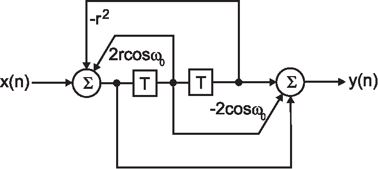
In order to obtain a data flow diagram we need to get powers of $z^{-1}$ because they represent delays.

  $$H(z) = \frac{1}{1 - 2 r \cos(\omega_{0}) z^{-1} + r^{2} z^{-2}}$$ (184)

which we multiply with the input signal $Y(z)$:

$$Y(z) = X(z) \frac{1}{1 - 2 r \cos (\omega) z^{-1} + r^{2} z^{-2}}$$ (185)

$$X(z) = Y(z) - Y(z) 2r \cos (\omega_{0}) z^{-1} + Y(z) r^{2} z^{-2}$$ (186)

$$Y(z) = X(z) + z^{-1} Y(z) 2r \cos (\omega_{0}) - z^{-2} Y(z) r^{2}$$ (187)

This gives us a second order recursive filter (IIR) which is shown in Fig 26. These complex conjugate poles generate a resonance at $\pm\omega_0$ where the amplitude is determined by $r$.

Stability

A transfer function $H(z)$ is only stable if the poles lie inside the unit circle. This is equivalent to the analog case where the poles of $H(s)$ have to lie on the left hand side of the complex plane (see Eq. 159). Looking at Eq. 183 it becomes clear that $r$ determines the radius of the two complex conjugate poles. If $r>1$ then the filter becomes unstable. The same applies to poles on the real axis. Their the real values have to stay within the range $-1 \ldots +1$.

In summary: poles generate resonances and amplify frequencies. The amplification is strongest the closer the poles move towards the unit circle. The poles need to stay within the unit circle to guarantee stability.

Note that in real implementations the coefficients of the filters are limited in precision. This means that a filter might work perfectly in python but will fail on a DSP with its limited precision. You can simlate this by forcing a certain datatype in python or you write it properly in C.

Poles and zeroes combined: design of a pure digital IIR notch filter

Figure 27: A two tap IIR bandstop filter with tuneable stopband width $r$ for the frequency $\omega _0$.

Now we combine the filters from the last two sections:

  $$H(z) = \frac {1 - 2 \cos (\omega_{0}) z^{-1} + z^{-2}}{1 - 2r \cos (\omega_{0}) z^{-1} + r^{2} z^{-2}}$$ (188)

This gives us a notch filter where its width is tunable with the help of $r<1$. The closer $r$ goes towards $1$ the more narrow is the frequency response. This filter has two poles and two zeros. The zeros sit on the unit circle and eliminate the frequencies $\pm\omega_0$ while the poles sit within the unit circle and generate a resonance around $\pm\omega_0$. As long as $r<1$ this resonance will not go towards infinity at $\pm\omega_0$ so that the zeros will always eliminate the frequencies $\pm\omega_0$.

Identifying filters from their poles and zeroes

Proakis and Manolakis (1996, pp.333) has an excellent section about this topic and we refer the reader to have a look. As a rule of thumb a digital lowpass filter has poles where their real parts are positive and a highpass filter has poles with negative real part of the complex poles. In both cases they reside within the unit circle to guarantee stability.

github / contact